Metatranscriptomics with Metagenomics
Protocol adapted from Guillem Salazar.
Metatranscriptomics is the analysis of all of the transcriptomes present in a sample and is an effective method to assess the activity of a microbial community. Unlike metagenomic data, metatranscriptomics can help decipher the metabolic functions actively expressed by the community at any given time.
Advantages:
Best way to get information about community activity.
Disadvantages:
Sample preparation might be difficult and expensive.
Data analysis methods are not well established.
Metatranscriptomic experiments can be broadly summarised into 2 different types: experiments that include matching metagenomic samples and those that do not. The analysis of these two datatypes are different. You can find a tutorial of how to analyze metatranscriptomic data without metagenomics on our Metatranscriptomics without Metagenomics (defined Community) website.
Dataset
Here, we will combine metatranscriptomics with metagenomics by using metagenomic data to normalize the transcript abundance. In order to do this, metagenomic data was processed as described in gene catalog creation to create a gene catalog. Gene functional annotation into orthologous groups was then performed using the KEGG database. The metagenomic data was then mapped back to the gene catalog to determine gene abundance. And the metatranscriptomic data from each sample was then mapped to the gene catalog to determine transcript abundance. To determine gene expression, we will look at the ratios of transcript abundance to gene abundance (after some normalisations of course).
Note
Transcript abundance depends on both gene abundance (number of genes) and expression level (number of mRNAs per gene). See Figure S1 for more information.
Note
The -1 fraction are unannotated genes, which we must account for, for proper normalisation. You can read more on this in the Gene length normalisation section.
The dataset used in this tutorial is from the article Gene Expression Changes and Community Turnover Differentially Shape the Global Ocean Metatranscriptome, Salazar et al.
The data can be downloaded here. These files are just a subset of the full dataset and are only meant to be used for this tutorial. To learn how to download and unpack the data follow these instructions.
This will contain the following files:
MGS_K03040_K03043_tara.tsv.gz contains a sample of raw counts for metagenomic and metatranscriptomic samples.
MGS_K03040_K03043_tara_lengthnorm.tsv.gz contains length normalised counts for metagenomic and metatranscriptomic samples.
K03704_tara_lengthnorm_percell.tsv.gz contains length and per-cell normalised counts for K03704 for metagenomic and metatranscriptomic samples.
sample_info.csv contains some metadata about the samples.
Data Normalisation
For both gene abundance and transcript abundance data, we must remove the following sources of bias:
Differences in gene length between genes.
Differences in sequencing depth between samples.
Differences in genome size distribution between samples.
Compositionality: The number of inserts for a given gene in a given sample can only be interpreted relative to the rest of the genes in the sample.
Note
Genome size differences can lead to biases and challenges in accurately comparing gene expression levels between different samples. To account for the genome size differences we will normalize the gene and transcript abundance data by abundances of 10 marker genes. This is explained in further detail in the section Sequencing depth, per cell normalisation and compositionality.
        flowchart LR
     id5(Gene count table) --> id1
     id6(Transcript count table) --> id1
     id1( Normalisation) --> id2(gene<br/>length<br/>normalisation)
     id2 --> id3(sequencing<br/>depth<br/>normalisation)
     id3 --> id4(per cell/<br/>normalisation)
     id4 --> id7(statistical analysis)
     classDef tool fill:#96D2E7,stroke:#F8F7F7,stroke-width:1px;
     style id1 fill:#5A729A,stroke:#F8F7F7,stroke-width:1px,color:#fff
     class id2,id3,id4,id7 tool
     style id5 fill:#F78A4A,stroke:#F8F7F7,stroke-width:1px
     style id6 fill:#F78A4A,stroke:#F8F7F7,stroke-width:1px
Setting up R environment and loading the data
We perform all of the normalisation steps in R. To run this analysis you will need tidyverse and data.table libraries.
library(data.table)
library(tidyverse)
# To read compressed files data.table needs R.utils library
library(R.utils)
library(patchwork)
library(GGally)
Next we are going to load gene and transcript abundances and metadata (i.e. temperature, location, depth, etc.).
# Load the gene and transcript abundances
profile <- fread("datasets/part1/MGS_K03040_K03043_tara.tsv.gz",sep="\t",
             header=T,data.table = F,tmpdir=".")
sample_info <- fread("datasets/part1/sample_info.csv",sep=",",
            header=T, data.table = F, tmpdir=".")
Gene length normalisation
The first step in the normalisation process is to divide the insert counts by the gene length for each gene in each sample. Since the unmapped (-1) fraction does not have a length, we assign it the median gene length.
Note
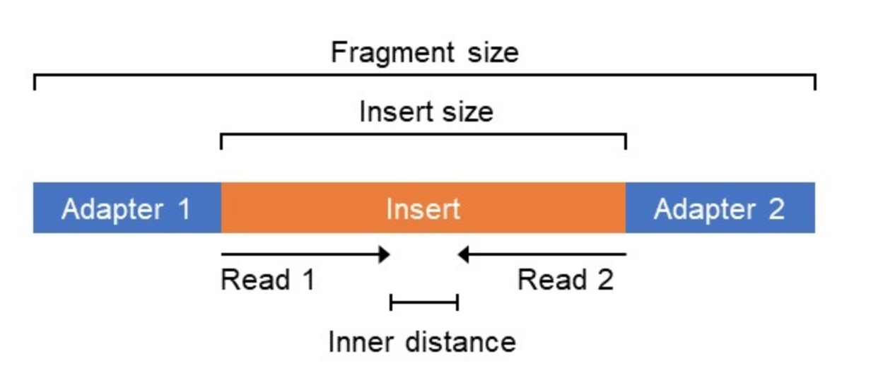
During short read sequencing, DNA is randomly sheared into inserts of known size distribution and sequenced. If paired-end sequencing is used, two DNA sequences (reads) are generated - one from each end of a DNA fragment. Here, we count inserts, not reads.
# Assigns median gene length to -1 fraction
# Example file does not contain -1 fraction, so this will have no effect for us
if (length(which(profile$length < 0)) > 0){
  med_length = median(profile$length[which(profile$length > 0)])
  profile$length[which(profile$length < 0)] <- med_length
}
We now build a gene-length normalized profile
profile_lengthnorm <- profile[, 1:4]
for (i in 5:ncol(profile)){
  cat("Normalizing by gene length: sample", colnames(profile)[i], "\n")
  tmp <- profile[, i]/profile$length %>%
    as.data.frame()
  colnames(tmp) <- colnames(profile)[i]
  profile_lengthnorm <- profile_lengthnorm %>%
    bind_cols(tmp)
}
Sequencing depth, per cell normalisation and compositionality
To account for differences in sequencing depth, as well as for differences in genome sizes between different samples,
Note
What are marker genes (MGs)?
Universal: present in “all” prokaryotes
Single-copy: always present once per cell (genome)
Are housekeeping genes
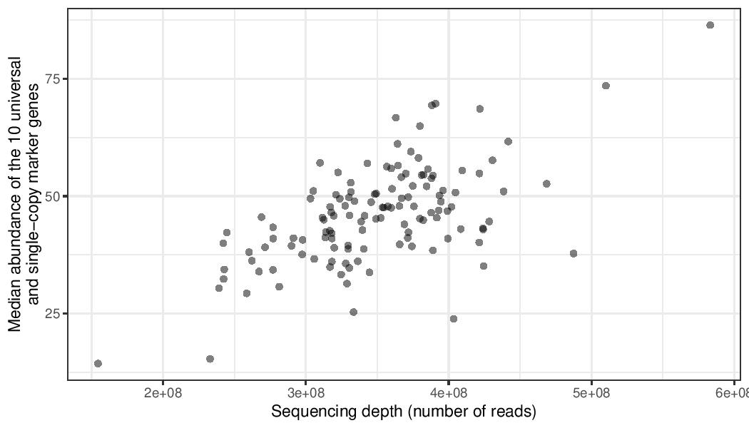
Because of these characteristics, the abundance of marker genes (MGs) correlates well with the sequencing depth. In addition, the median abundance of MGs is a good proxy for the number of cells captured in a given metagenomic/metatranscriptomic sample. The per-cell normalization accounts for differences in genome sizes between samples and also controls for compositionality. The result of this normalisation is a biologically meaningful unit: gene copies per total cell in the community.
To normalize by abundance of 10 MGs, we first compute their total insert count in each sample (i.e. sum the counts for each of the 10 KOs). We then compute the median of the 10 MGs in each sample. Finally, we divide the gene-length normalized abundances by this median for each sample.
In this example we use the following marker genes:
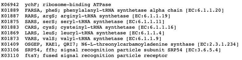
# Define the KOs corresponding to the 10 MGs
mgs <- c("K06942", "K01889", "K01887", "K01875", "K01883",
         "K01869", "K01873", "K01409", "K03106", "K03110")


# Build a MGs normalized profile
profile_lengthnorm_mgnorm <- profile_lengthnorm[, 1:4]

for (i in 5:ncol(profile_lengthnorm)){
  cat("Normalizing by 10 MGs: sample", colnames(profile_lengthnorm)[i], "\n")
  mg_median <- profile_lengthnorm %>%
    select(KO, abundance = all_of(colnames(profile_lengthnorm)[i])) %>%
    filter(KO %in% mgs) %>%
    group_by(KO) %>% summarise(abundance = sum(abundance)) %>%
    ungroup() %>% summarise(mg_median = median(abundance)) %>%
    pull()
  tmp <- profile_lengthnorm[,i]/mg_median
  tmp <- tmp %>% as.data.frame()
  colnames(tmp) <- colnames(profile_lengthnorm)[i]
  profile_lengthnorm_mgnorm <- profile_lengthnorm_mgnorm %>%
    bind_cols(tmp)
}
Showing the effect of the normalization
Here, we visualize the effect of the normalization based on length and abundance of marker genes. Using this script we create the following plots:
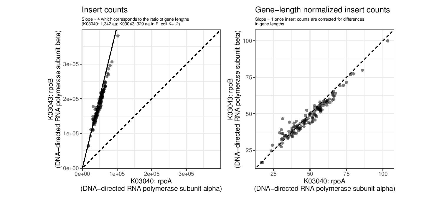
We will first look at 2 KOs: K03040 and K03043. These encode for 2 subunits of RNA polymerase. We first subset the raw metagenomic counts for these 2 genes (rp_ab) and then do the same with length normalised counts (rp_ab_lengthnorm), and finally visualize the relationship.
# Compute the abundance of K03040 and K03043 with and without gene-length normalization
rp_ab <- profile %>%
  select(-reference, -length, -Description) %>%
  filter(KO %in% c("K03040", "K03043")) %>%
  pivot_longer(-KO, names_to = "sample", values_to = "inserts") %>%
  filter(grepl('METAG', sample)) %>%
  group_by(KO, sample) %>% summarize(inserts = sum(inserts)) %>%
  pivot_wider(names_from = "KO", values_from = "inserts")

rp_ab_lengthnorm <- profile_lengthnorm %>%
  select(-reference, -length, -Description) %>%
  filter(KO %in% c("K03040", "K03043")) %>%
  pivot_longer(-KO, names_to = "sample", values_to = "inserts_lengthnorm") %>%
  filter(grepl('METAG', sample)) %>%
  group_by(KO, sample) %>% summarise(inserts_lengthnorm = sum(inserts_lengthnorm)) %>%
  pivot_wider(names_from = "KO", values_from = "inserts_lengthnorm")


g1 <- ggplot(data = rp_ab, aes(x = K03040, y = K03043)) +
  geom_point(alpha = 0.5) +
  geom_abline(slope = (1342/329)) +
  geom_abline(linetype = 2) +
  xlim(range(rp_ab$K03040, rp_ab$K03043)) +
  ylim(range(rp_ab$K03040, rp_ab$K03043)) +
  xlab("K03040: rpoA\n(DNA-directed RNA polymerase subunit alpha)") +
  ylab("K03043: rpoB\n(DNA-directed RNA polymerase subunit beta)") +
  labs(title = "Insert counts", subtitle = "Slope ~ 4 which corresponds to the ratio of gene lengths\n(K03040: 1,342 aa; K03043: 329 aa in E. coli K-12)") +
  coord_fixed() +
  theme_bw() +
  theme(plot.subtitle = element_text(size = 7))


g2 <- ggplot(data = rp_ab_lengthnorm, aes(x = K03040, y = K03043)) +
  geom_point(alpha = 0.5) +
  geom_abline(linetype = 2) +
  xlim(range(rp_ab_lengthnorm$K03040, rp_ab_lengthnorm$K03043)) +
  ylim(range(rp_ab_lengthnorm$K03040, rp_ab_lengthnorm$K03043)) +
  xlab("K03040: rpoA\n(DNA-directed RNA polymerase subunit alpha)") +
  ylab("K03043: rpoB\n(DNA-directed RNA polymerase subunit beta)") +
  labs(title = "Gene-length normalized insert counts", subtitle = "Slope ~ 1 once insert counts are corrected for differences\nin gene lengths") +
  coord_fixed() +
  theme_bw() +
  theme(plot.subtitle = element_text(size = 7))

g1|g2
Now, we’re going to look at correlation of marker gene abundance with sequencing depth and the correlation in abundance between different marker genes.
# Compute the abundance of the 10MGs and correlate to sequencing depth
mgs_ab_lengthnorm <- profile_lengthnorm %>%
select(-reference, -Description, -length) %>%
filter(KO %in% mgs) %>%
pivot_longer(-KO, names_to = "sample", values_to = "inserts_lengthnorm") %>%
group_by(KO, sample) %>% summarise(inserts_lengthnorm = sum(inserts_lengthnorm)) %>%
ungroup() %>% group_by(sample) %>% summarise(median_mgs = median(inserts_lengthnorm)) %>%
inner_join(sample_info, by = c("sample" = "sample_metag"))
g3 <- ggplot(data = mgs_ab_lengthnorm, aes(x = sample_metag_nreads, y = median_mgs)) +
geom_point(alpha = 0.5) +
#geom_smooth(method = "lm") +
#scale_x_log10() +
#scale_y_log10() +
xlab("Sequencing depth (number of reads)") +
ylab("Median abundance of the 10 universal\nand single-copy marker genes") +
theme_bw() +
theme(legend.title = element_blank())
g3
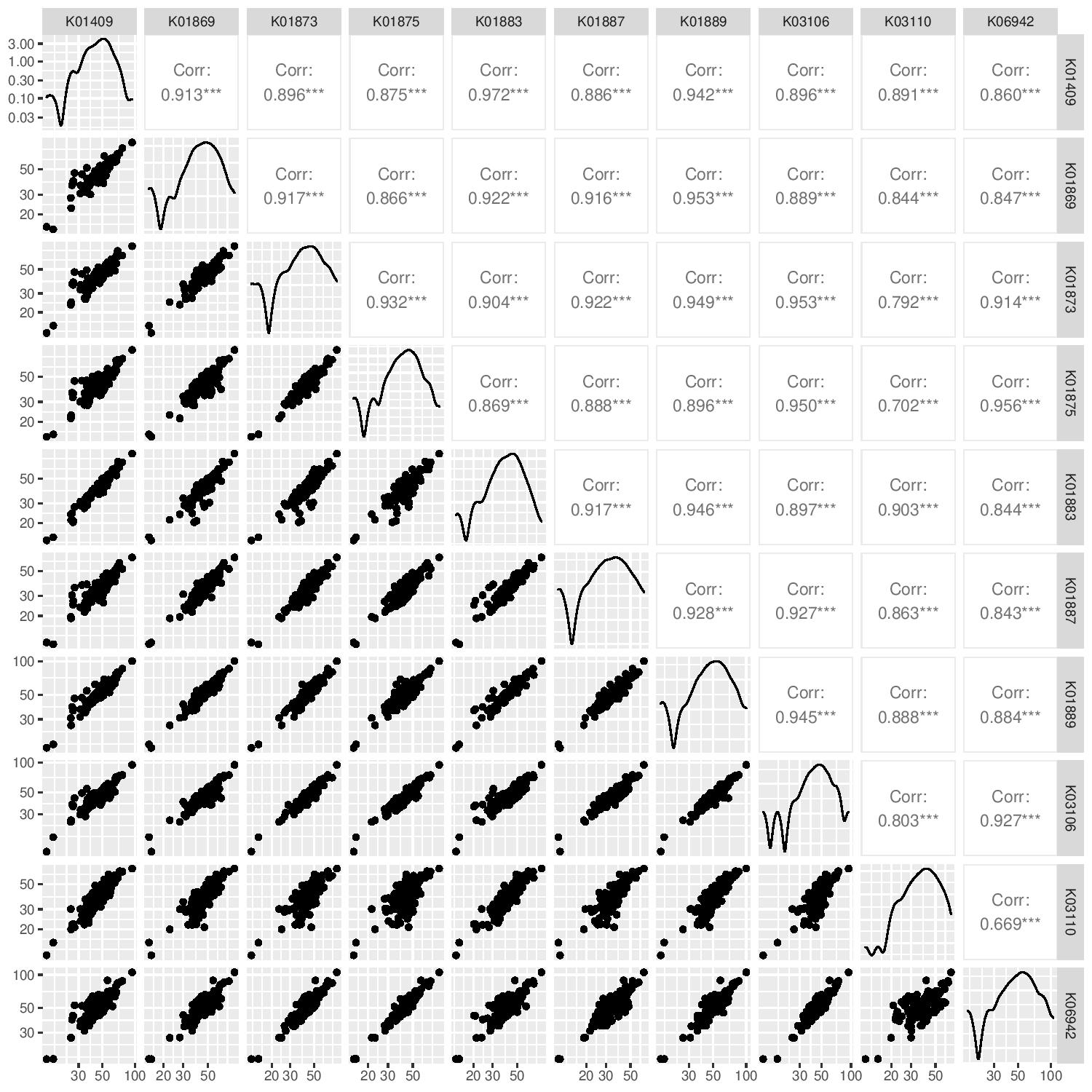
# Compute the abundance of the 10MGs and their autocorrelation
mgs_ab_lengthnorm <- profile_lengthnorm %>%
select(-reference, -Description, -length) %>%
filter(KO %in% mgs) %>%
pivot_longer(-KO, names_to = "sample", values_to = "inserts_lengthnorm") %>%
group_by(KO, sample) %>% summarise(inserts_lengthnorm = sum(inserts_lengthnorm)) %>%
inner_join(sample_info, by = c("sample" = "sample_metag")) %>%
select(KO, sample, inserts_lengthnorm) %>%
pivot_wider(names_from = "KO", values_from = "inserts_lengthnorm")
g4 <- ggpairs(data = mgs_ab_lengthnorm %>% column_to_rownames("sample")) +
scale_x_log10() +
scale_y_log10()
g4
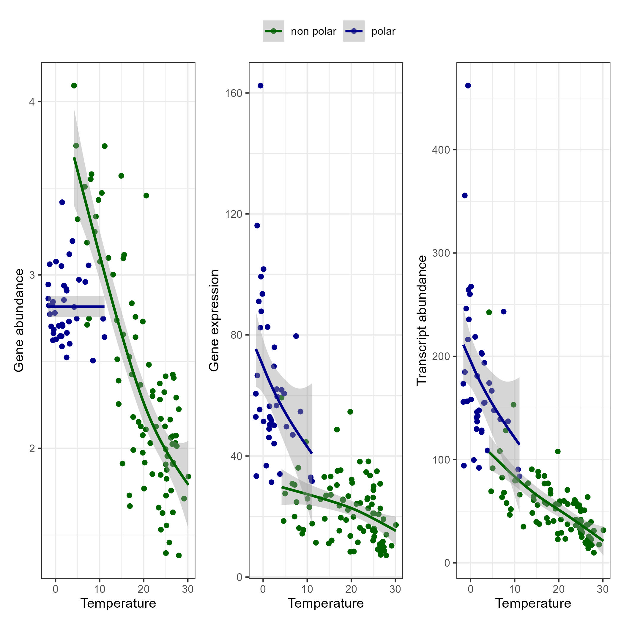
Combining Metatranscriptomic and Metagenomic Data
In this section we combine metatranscriptomic and metagenomic data and create the following plot:
# Load normalized profile
gc_profile <- fread("datasets/part1/K03704_tara_lengthnorm_percell.tsv.gz", sep = "\t", header = T, data.table = F, tmpdir = ".")
sample_info <- fread("datasets/part1/sample_info.csv",sep=",",
            header=T, data.table = F, tmpdir=".")


ko_profile <- gc_profile %>%
  group_by(KO) %>% summarise(across(starts_with("TARA"), sum)) %>%
  as.data.frame()


# Compute the gene abundance, transcript abundance and expression for the pairs of metaG-metaT samples
# The expression is just the ratio of transcript_abundance to gene_abundance
tmp_sample_info <- sample_info %>%
  select(sample_metag, sample_metat) %>%
  mutate(sample_pair = paste(sample_metag, sample_metat, sep = "-"))
tmp_metag <- ko_profile %>%
  select(KO, all_of(tmp_sample_info$sample_metag)) %>%
  pivot_longer(-KO, names_to = "sample_metag", values_to = "gene_abundance")
tmp_metat <- ko_profile %>%
  select(KO, all_of(tmp_sample_info$sample_metat)) %>%
  pivot_longer(-KO, names_to = "sample_metat", values_to = "transcript_abundance")
final_profile <- tmp_sample_info %>%
  left_join(tmp_metag, by = "sample_metag") %>%
  left_join(tmp_metat, by = c("KO", "sample_metat")) %>%
  mutate(expression = transcript_abundance/gene_abundance)

toplot <- final_profile %>%
  filter(KO == "K03704") %>%
  left_join(sample_info, by = c("sample_metag","sample_metat"))

g_metat <- ggplot(data = toplot, aes(y = transcript_abundance, x = Temperature, color =  polar)) +
  geom_point() +
  geom_smooth(method = "gam", se = T, formula = y ~ s(x, bs = "cs", k=5)) +
  scale_color_manual(values = c("darkgreen", "darkblue"))+
  ylab("Transcript abundance") +
  theme_bw() +
  theme(legend.position = "none")
g_metag <- ggplot(data = toplot, aes(y = gene_abundance, x = Temperature, color = polar)) +
  geom_point() +
  geom_smooth(method = "gam", se = T, formula = y ~ s(x, bs = "cs", k=5)) +
  #scale_y_log10() +
  #coord_flip() +
  scale_color_manual(values = c("darkgreen", "darkblue")) +
  ylab("Gene abundance") +
  theme_bw() +
  theme(legend.position = "none")
g_exp <- ggplot(data = toplot, aes(y = expression, x = Temperature, color = polar)) +
  geom_point() +
  geom_smooth(method = "gam", se = T, formula = y ~ s(x, bs = "cs", k=5)) +
  #scale_y_log10() +
  #coord_flip() +
  scale_color_manual(values = c("darkgreen", "darkblue")) +
  ylab("Gene expression") +
  theme_bw() +
  theme(legend.position = "top", legend.title = element_blank())
g <- g_metag | g_exp | g_metat
g