Metagenomic Assembly
Protocol provided by Hans-Joachim Ruscheweyh.
Technical advances in sequencing technologies in recent decades have allowed detailed investigation of complex microbial communities without the need for cultivation. Sequencing of microbial DNA extracted directly from environmental or host-associated samples have provided key information on microbial community composition. These studies have also allowed gene-level characterization of microbiomes as the first step to understanding the communities’ functional potential. Furthermore, algorithmic improvements, as well as increased availability of computational resources, make it now possible to reconstruct whole genomes from metagenomic samples (metagenome-assembled genomes (MAGs)). Methods for microbial community composition analysis are discussed in Taxonomic Profiling of Metagenomes. Here, we describe building Metagenomic Assembly as well as building Gene Catalogs and MAGs from metagenomic data.
Note
Sample data and conda environment file for this section can be found here. See the Tutorials section for instructions on how to unpack the data and create the conda environment. After unpacking the data, run cd metag_test, and you should see conda specifications metag.yaml and a reads directory containing a set of forward (.1.fq.gz) and reverse (.2.fq.gz) reads for 3 metagenomic samples. These reads have already been through the Data Preprocessing workflow and can be used directly for metagenomic assembly. There should also be scaffolds_filter.py.
Metagenomic Assembly
        flowchart LR
     id1( Metagenomic<br/>Assembly) --> id2(data preprocessing)
     id2 --> id3(metagenomic assembly<br/>fa:fa-cog metaSPAdes)
     id3 --> id4(gene catalogs)
     id3 --> id5(MAGs)
     classDef tool fill:#96D2E7,stroke:#F8F7F7,stroke-width:1px;
     style id1 fill:#5A729A,stroke:#F8F7F7,stroke-width:1px,color:#fff
     style id2 fill:#F78A4A,stroke:#F8F7F7,stroke-width:1px
     class id3,id4,id5 tool
Data Preprocessing. Before proceeding to the assembly, it is important to preprocess the raw sequencing data. Standard preprocessing protocols are described in Data Preprocessing. In addition to standard quality control and adapter trimming, we also suggest normalization with bbnorm.sh and merging of paired-end reads (see Data Preprocessing for more details).
Metagenomic Assembly. Following data preprocessing, we use clean reads to perform a metagenomic assembly using metaSPAdes. metaSPAdes is part of the SPAdes assembly toolkit. Following the assembly, we generate some assembly statistics using assembly-stats, and filter out contigs that are < 1 kbp in length. The script we use for scaffold filtering can be found here:
scaffold_filter.py. It is also included in the test dataset for this section.
Assembly:
mkdir metag_assembly
for i in 1 2 3
  do
    mkdir metag_assembly/metag$i
    metaspades.py -t 4 -m 10 --only-assembler \
    --pe1-1 reads/metag$i.1.fq.gz \
    --pe1-2 reads/metag$i.2.fq.gz \
    -o metag_assembly/metag$i
  done
|
Number of threads |
|
Set memory limit in Gb; spades will terminate if that limit is reached |
|
Run assembly module only (spades can also perform read error correction, this step will be skipped) |
|
Forward reads |
|
Reverse reads |
|
Unpaired reads |
|
Merged reads |
|
Specify output directory |
Computational Resources needed for metagenomic assembly will vary significantly between datasets. In general, metagenomic assembly requires a lot of memory (usually > 100 Gb). You can use multiple threads (16-32) to speed up the assembly. Because test data set provided is very small, merging of the pair-end reads was not necessary (see Data Preprocessing). It is helpful when working with real data - don’t forget to include the merged and singleton files with
--pe1-mand--pe1-soptions.
Filtering:
Assumes scaffolds_filter.py is in metag_test
cd metag_assembly
for i in 1 2 3
  do
    python ../scaffold_filter.py metag$i scaffolds metag$i/scaffolds.fasta metag$i META
  done
|
Sample name |
|
Sequence type (can be contigs, scaffolds or transcripts) |
|
Input assembly to filter |
|
Prefix for the output file |
|
Type of assembly (META for metagenomics or ISO for isolate genomes) |
Stats:
for i in 1 2 3
  do
    assembly-stats -l 500 -t <(cat metag$i/metag$i.scaffolds.min500.fasta) \
    > metag$i/metag$i.assembly.stats
  done
|
Minimum length cutoff for each sequence |
|
Print tab-delimited output |
The metagenomic scaffolds generated in step 2 can now be used to build and/or profile Gene Catalogs or to construct MAGs.
Gene Catalogs
Gene catalog generation and profiling (i.e. gene abundance estimation) can provide important insights into the community’s structure, diversity and functional potential. This analysis could also identify relationships between genetic composition and environmental factors, as well as disease associations.
Note
Integrated catalogs of reference genes have been generated for many ecosystems (e.g. ocean, human gut, and many others) and might be a good starting point for the analysis.
Building
This protocol will allow you to create a de novo gene catalog from your metagenomic samples.
        flowchart LR
     id1( Building a<br/>Gene Catalog) ---> id2(gene calling<br/>fa:fa-cog prodigal)
     id2 ---> id3(gene dereplication<br/>fa:fa-cog CD-HIT)
     classDef tool fill:#96D2E7,stroke:#F8F7F7,stroke-width:1px;
     style id1 fill:#5A729A,stroke:#F8F7F7,stroke-width:1px,color:#fff
     class id2,id3 tool
Gene calling. We use prodigal to extract protein-coding genes from metagenomic assemblies (using scaffolds >= 500 bp as input). Prodigal has different gene prediction modes with single genome mode as default. To run prodigal on metagenomic data, we add the
-p metaoption. This will produce a fasta file with amino acid sequences (.faa), nucleotide sequences (.fna) for each gene, as well as an annotation file (.gff).
Gene Calling
Assumes you are in the metag_assembly directory.
for i in 1 2 3
  do
    prodigal -a metag$i/metag$i.faa -d metag$i/metag$i.fna -f gff \
    -o metag$i/metag$i.gff -c -q -p meta \
    -i metag$i/metag$i.scaffolds.min500.fasta
  done
|
Specify protein translations file |
|
Specify nucleotide sequences file |
|
Specify output format: gbk: Genbank-like format (Default); gff: GFF format; sqn: Sequin feature table format; sco: Simple coordinate output |
|
Specify output file, default stdout |
|
Closed ends, do not allow partial genes at edges of sequence |
|
Run quietly (suppress logging output) |
|
Specify mode: single or meta |
|
Input FASTA or Genbank file |
Gene de-replication. At this point gene-nucleotide sequences from all samples are concatenated together and duplicated sequences are removed from the catalog. For this, genes are clustered at 95% identity and 90% coverage of the shorter gene using CD-HIT. The longest gene sequence from each cluster is then used as a reference sequence for this gene.
Clustering
cd ..
mkdir gene_catalog
cat metag_assembly/metag*/metag*fna > gene_catalog/gene_catalog_all.fna
cat metag_assembly/metag*/metag*faa > gene_catalog/gene_catalog_all.faa
cd gene_catalog
mkdir cdhit9590
cd-hit-est -i gene_catalog_all.fna -o cdhit9590/gene_catalog_cdhit9590.fasta \
-c 0.95 -T 64 -M 0 -G 0 -aS 0.9 -g 1 -r 1 -d 0
|
Input filename in fasta format, required |
|
Output filename, required |
|
Sequence identity threshold, default 0.9 |
|
Number of threads, default 1; with 0, all CPUs will be used |
|
Memory limit (in MB) for the program, default 800; 0 for unlimited |
|
Use global sequence identity, default 1; if set to 0, then use local sequence identity, don’t use -G 0 unless you use alignment coverage controls (e.g. options -aS) |
|
Alignment coverage for the shorter sequence, default 0.0; if set to 0.9, the alignment must cover 90% of the sequence |
|
1 or 0, default 0; by cd-hit’s default algorithm, a sequence is clustered to the first cluster that meets the threshold (fast cluster); if set to 1, the program will cluster it into the most similar cluster that meets the threshold (accurate but slow mode); either 1 or 0 won’t change the representatives of final clusters |
|
1 or 0, default 1; by default do both +/+ & +/- alignments; if set to 0, only +/+ strand alignment |
|
length of description in .clstr file, default 20; if set to 0, it takes the fasta defline and stops at first space |
The fasta file generated by CD-HIT will contain a representative sequence for each gene cluster. To extract protein sequences for each gene in the catalog, we first extract all the sequence identifiers from the CD-HIT output file and use seqtk subseq command to extract these sequences from gene_catalog_all.faa. This file can be then used for downstream analysis (ex. KEGG annotations).
grep "^>" cdhit9590/gene_catalog_cdhit9590.fasta | \
cut -f 2 -d ">" | \
cut -f 1 -d " " > cdhit9590/cdhit9590.headers
seqtk subseq gene_catalog_all.faa cdhit9590/cdhit9590.headers \
> cdhit9590/gene_catalog_cdhit9590.faa
Gene Catalog Profiling
Warning
Incomplete protocol
        flowchart LR
     id1( Gene Catalog<br/>Profiling) --> id2(read alignment<br/>fa:fa-cog BWA)
     id2 --> id3(filtering<br/>the alignment files<br/>fa:fa-ban)
     id3 --> id4(counting<br/>gene abundance<br/>fa:fa-ban)
     classDef tool fill:#96D2E7,stroke:#F8F7F7,stroke-width:1px;
     style id1 fill:#5A729A,stroke:#F8F7F7,stroke-width:1px,color:#fff
     class id2,id3,id4 tool
This protocol allows quantification of genes in a gene catalog for each metagenomic sample.
Read alignment. In the first step, (cleaned) sequencing reads are mapped back to the gene catalog using BWA aligner. Note that forward, reverse, singleton and merged reads are mapped separately and are then filtered and merged in a later step.
Alignment
Make sure you are back in metag_test directory. Note that test data do not include merged and singleton files. If you have those, do not forget to align those separately as well.
mkdir alignments
bwa index gene_catalog/cdhit9590/gene_catalog_cdhit9590.fasta

bwa mem -a -t 4 gene_catalog/cdhit9590/gene_catalog_cdhit9590.fasta reads/metag1.1.fq.gz \
| samtools view -F 4 -bh - > alignments/metag1.r1.bam

bwa mem -a -t 4 gene_catalog/cdhit9590/gene_catalog_cdhit9590.fasta reads/metag1.2.fq.gz \
| samtools view -F 4 -bh - > alignments/metag1.r2.bam
BWA:
|
Output all found alignments for single-end or unpaired paired-end reads, these alignments will be flagged as secondary alignments |
|
Number of threads |
samtools:
|
Do not output alignments with any bits set in FLAG present in the FLAG field. When FLAG is 4, do not output unmapped reads. |
|
Output in the BAM format |
|
Include the header in the output |
Filtering the alignment files. To make sure that quantification of gene abundance relies only on high confidence alignments, the alignment files are first filtered to only include alignments with length > 45 nt and percent identity > 95%.
Counting gene abundance. This step counts the number of reads aligned to each gene for each of the samples.
Important
We’re currently working on a tool that can merge and filter alignment files, as well as quantify gene abundances. Stay tuned! In the meanwhile, please contact us to learn more.
Note
Gene catalogs and collections of MAGs are often used to infer abundance of microorganisms in metagenomic samples, however none are comprehensive and will miss some members (or the majority) of the microbial community. It is important to estimate what percentage of the microbial community is represented in a gene catalog or a collection of MAGs. This is evaluated using mapping rates: number of mapped reads (after alignment and filtering, as described in Gene Catalog Profiling) divided by total number of quality-control reads.
Important
Per-cell normalization. Metagenomic profiles should be normalized to relative cell numbers in the sample. This can be achieved by dividing the gene abundances by the median abundance of 10 universal single-copy phylogenetic marker genes (MGs).
MAGs
The Holy Grail of metagenomics is to be able to assemble individual microbial genomes from complex community samples. However, short-read assemblers fail to reconstruct complete genomes. For that reason, binning approaches have been developed to facilitate creation of Metagenome Assembled Genomes (MAGs).
MAG reconstruction algorithms have to decipher which of the scaffolds generated during Metagenomic Assembly belong to the same organism (referred to as bin). While different binning approaches have been described, here we use MetaBAT2 for MAG reconstruction. As shown in the figure below, MetaBAT2 uses scaffolds’ tetranucleotide frequencies and abundances to group scaffolds into bins.
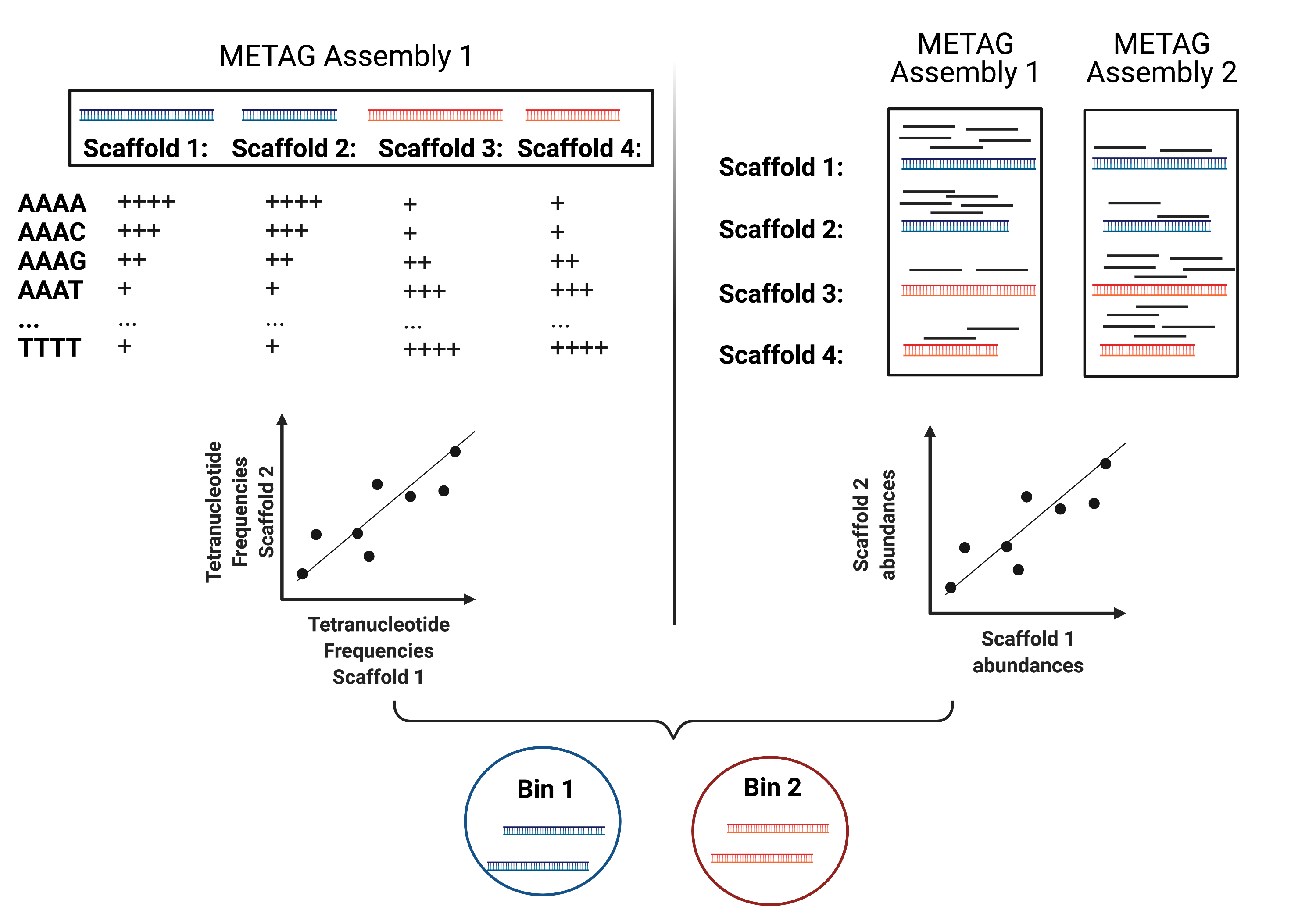
In this (very) simplified example, the blue scaffolds show similar tetranucleotide frequencies and similar abundances (across multiple samples), and consequently end up binned together, and separately from the red scaffolds.
MAG Building
        flowchart LR
     id1(MAGs) --> id2(all-to-all <br/>alignment<br/>fa:fa-cog BWA)
     id2 --> id3(within- and<br/>between-sample<br/>abundance correlation<br/>for each scaffold<br/>fa:fa-cog MetaBAT2 )
     id3 --> id4(metagenomic<br/>binning<br/>fa:fa-cog MetaBAT2)
     id4 --> id5(quality control<br/>fa:fa-cog CheckM)
     classDef tool fill:#96D2E7,stroke:#F8F7F7,stroke-width:1px;
     style id1 fill:#5A729A,stroke:#F8F7F7,stroke-width:1px,color:#fff
     class id2,id3,id4,id5 tool
This workflow starts with size-filtered metaSPAdes assembled scaffolds (resulted from Metagenomic Assembly). Note that for MAG building we are using >= 1000 bp scaffolds.
All-to-all alignment. In this step, quality controlled reads for each of the metagenomic samples are mapped to each of the metagenomic assemblies using BWA. Here, we use
-ato allow mapping to secondary sites. Note that merged, singleton, forward and reverse reads are all aligned separately, and are later merged into a singlebamfile.
Important
For MAG construction, the generated alignment files are filtered to only include alignments that are at least 45 nucleotides long, with an identity of >= 95 and covering 80% of the read sequence. The alignment filtering was done with a tool we are building in the lab and is not included in the example command below. Please contact us to learn more.
Create BWA index for each assembly:
Make sure you are in the metag_test directory and have run metagenomic assembly steps described above.
for i in 1 2 3
  do
    bwa index metag_assembly/metag$i/metag$i.scaffolds.min1000.fasta
  done
Mapping every sample to every assembly:
mkdir -p alignments
for i in 1 2 3
  do
    for j in 1 2 3
      do
        bwa mem -a -t 16 metag_assembly/metag$i/metag$i.scaffolds.min1000.fasta reads/metag$j.1.fq.gz \
        | samtools view -F 4 -bh - | samtools sort -O bam -@ 4 -m 4G > alignments/metag"$j"_to_metag"$i".1.bam
        bwa mem -a -t 16 metag_assembly/metag$i/metag$i.scaffolds.min1000.fasta reads/metag$j.2.fq.gz \
        | samtools view -F 4 -bh - |samtools sort -O bam -@ 4 -m 4G > alignments/metag"$j"_to_metag"$i".2.bam
        samtools merge alignments/metag"$j"_to_metag"$i".bam \
        alignments/metag"$j"_to_metag"$i".1.bam alignments/metag"$j"_to_metag"$i".2.bam
      done
  done
BWA:
|
Output all found alignments for single-end or unpaired paired-end reads, these alignments will be flagged as secondary alignments |
|
Number of threads |
samtools:
|
Do not output alignments with any bits set in FLAG present in the FLAG field. When FLAG is 4, do not output unmapped reads. |
|
Output in the BAM format |
|
Include the header in the output |
Important
Computational Resources: Depending on the size of the dataset, this step would require significant computational resources.
Within- and between-sample abundance correlation for each contig. MetaBAT2 provides jgi_summarize_bam_contig_depth script that allows quantification of within- and between-sample abundances for each scaffold. Here, we generate an abundance (depth) file for each metagenomic assembly by providing the alignment files generated using this assembly. This depth file will be used by MetaBAT2 in the next step for scaffold binning.
Depth calculation:
for i in 1 2 3
  do
    jgi_summarize_bam_contig_depths --outputDepth alignments/metag$i.depth \
    alignments/metag*_to_metag"$i".bam
  done
Note
Binning with MetaBAT2 can also be accomplished without between-sample abundance correlation, however this step significantly improves the quality of reconstructed MAGs, and, in our opinion, is worth the computational burden of all-to-all alignment.
Metagenomic Binning. Finally, we run MetaBAT2 to bin the metagenomic assemblies using depth files generated in the previous step.
mkdir mags
for i in 1 2 3
  do
    metabat2 -i metag_assembly/metag$i/metag$i.scaffolds.min1000.fasta -a alignments/metag$i.depth \
    -o mags/metag$i --minContig 2000 \
    --maxEdges 500 -x 1 --minClsSize 200000 --saveCls -v
  done
Quality Control. After MAG reconstruction, it is important to estimate how well the binning perform. CheckM places each bin on a reference phylogenetic tree and evaluates genome quality by looking at a set of clade-specific marker genes. CheckM outputs completeness (estimation of fraction of genome present), contamination (percentage of foreign scaffolds), and strain heterogeneity (high strain heterogeneity would suggest that contamination is due to presence of closely related strains in your sample).
Warning
Linux only!
checkm lineage_wf mags mags -x fa \
-f mags/checkm_summary.txt --tab_table
MAG building: low abundance metagenome/pooled assembly
Warning
Under construction