Genome Assembly

Protocol provided by Anna Sintsova.

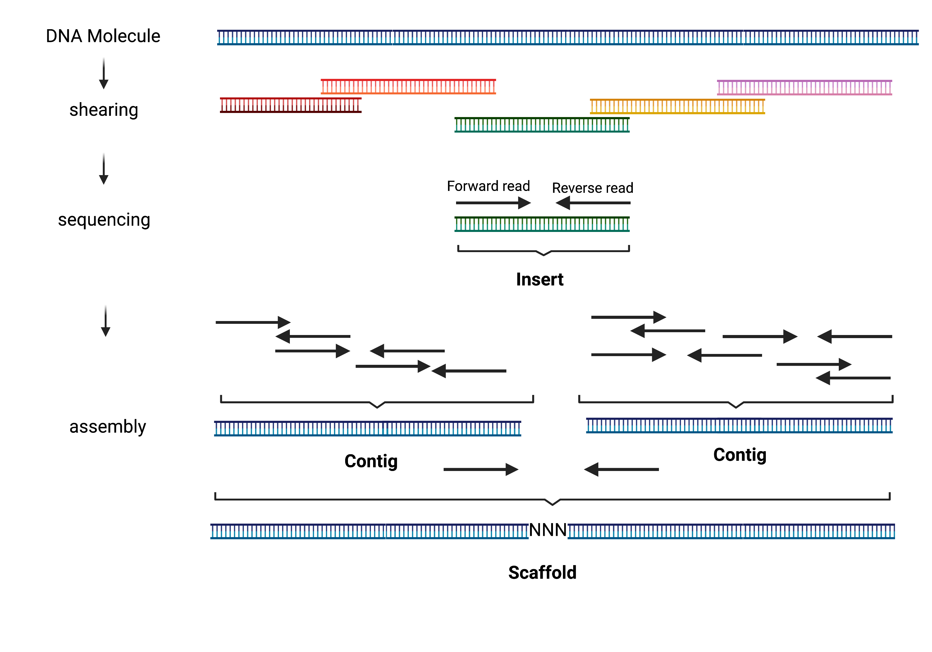
Over the recent years, bacterial whole genome sequencing has become an indispensable tool for microbiologists. While powerful, short read sequencing technologies only allow assembly of draft genomes (i.e. assembly consisting of multiple scaffolds). As illustrated below, during whole genome shotgun sequencing, DNA is randomly sheared into inserts of known size distribution and sequenced. If paired-end sequencing is used, two DNA sequences (reads) are generated - one from each end of a DNA fragment). The assemblers look for overlaps between sequencing reads to stitch them together into contigs. The contigs can then sometimes be linked together into longer scaffolds (for example with information from mate-pair reads).

Note

Long read sequencing (with PacBio or Nanopore) offers creation of complete circularized bacterial genomes. However, the bioinformatics methods for this are still in development. They are likely to change as technology develops, and the standard protocols are less well established (See this genome assembly guide for current suggestions).

Isolate genome assembly using short reads

flowchart LR id1( Isolate Genome<br/>Assembly) --> id2(data<br/>preprocessing<br/>fa:fa-cog optional: mOTUs) id2 --> id3(genome<br/>assembly<br/>fa:fa-cog SPAdes) id3 --> id4(assembly quality<br/>control<br/>fa:fa-cog QUAST<br/>fa:fa-cog assembly-stats) id4 --> id5(genome<br/>annotation<br/>fa:fa-cog prokka) classDef tool fill:#96D2E7,stroke:#F8F7F7,stroke-width:1px; style id1 fill:#5A729A,stroke:#F8F7F7,stroke-width:1px,color:#fff style id2 fill:#F78A4A,stroke:#F8F7F7,stroke-width:1px class id3,id4,id5 tool

Note

Sample data for this section can be found here. The conda environment specifications are here. See the Tutorials section for instructions on how to unpack the data and create the conda environment. After unpacking the data, you should have a set of forward (Sample1_R1.fq.gz) and reverse (Sample1_R2.fq.gz) reads. These reads have already been through the Data Preprocessing workflow and can be used directly for genome assembly. (Note: The included files adapters.fa and phix174_ill.ref.fa.gz are not needed here.)

1. Data Preprocessing. Before proceeding to the assembly, it is important to preprocess the raw sequencing data. Standard preprocessing protocols are described in Data Preprocessing. In addition to standard quality control and adapter trimming, we also suggest normalization with bbnorm.sh and merging (see Data Preprocessing for more details). Besides the common preprocessing steps, we usually run mOTUs on the cleaned sequencing reads, to check for sample contamination or mis-labelling (both occur more frequently than you would expect). For more details please check the Taxonomic Profiling of Metagenomes section.

2. Genome Assembly. Following data preprocessing, we assemble the cleaned reads using SPAdes. While SPAdes generated scaffolds using paired end data (i.e. no mate-pair libraries), there will be few differences between scaffolds.fasta and contigs.fasta. We use scaffolds for all subsequent analysis.

Example Command

mkdir sample1_assembly; \
spades.py -t 4 --isolate --pe1-1 Sample1_R1.fq.gz \
--pe1-2 Sample1_R2.fq.gz  -o sample1_assembly

-t	Number of threads
--isolate	Use SPAdes isolate mode
--pe1-1	Forward reads
--pe1-2	Reverse reads
-o	Specify output directory

3. Assembly Quality Control. Following assembly, we generate assembly statistics using assembly-stats, and filter out scaffolds that are < 500 bp in length. The script we use for contig/scaffold filtering can be found here: scaffold_filter.py. Alternatively, the metrics to evaluate genome quality can be also calculated using QUAST. The output will contain information on the number of contigs, the largest contig, total length of the assembly, GC%, N50, L50 and others. If reference genome assembly is available, QUAST will also assess misassemblies and try to categorize them.

Note

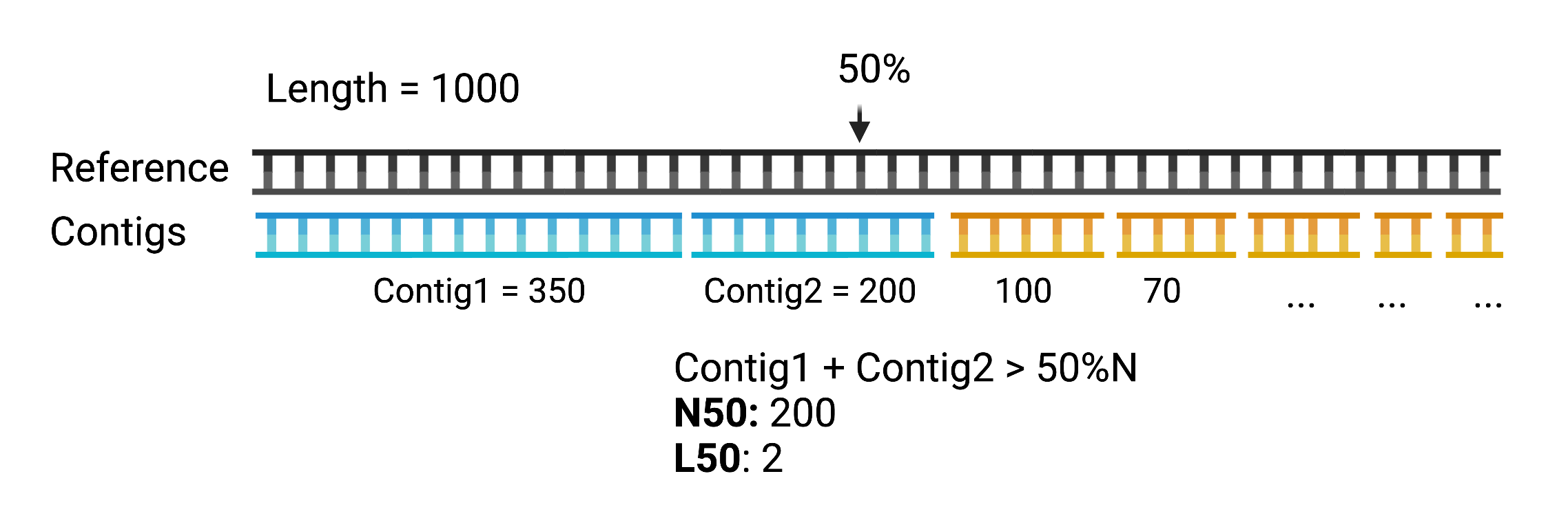
N50 and L50: Given a set of contigs sorted by length in descending order, L50 is the smallest number of contigs, whose length adds up to at least 50% of the genome length. N50 is the length of the smallest contig included in L50 (i.e. if L50 is 2, N50 will be length of the 2nd contig).

Example Command for filtering and stats:

python scaffold_filter.py Sample1 scaffolds \
sample1_assembly/scaffolds.fasta sample1_assembly ISO;
assembly-stats -l 500 \
-t sample1_assembly/Sample1.scaffolds.min500.fasta > \
sample1_assembly/Sample1.assembly.stats

Sample1	Sample name
scaffolds	Sequence type (can be contigs, scaffolds or transcripts)
sample1_assembly/scaffolds.fasta	Input assembly to filter
sample1_assembly	Prefix for the output file
ISO	Type of assembly (ISO for metagenomics or META for isolate genomes

Example QUAST Command:

quast.py sample1_assembly/Sample1.scaffolds.min500.fasta \
-1 Sample1_R1.fq.gz -2 Sample1_R2.fq.gz -o sample1_assembly

Options Explained

-1 (or --pe1)	File with forward paired-end reads in FASTQ format (files compressed with gzip are allowed).
-2 (or --pe2)	File with reverse paired-end reads in FASTQ format (files compressed with gzip are allowed).
-o	Specify output directory

4. Gene Calling and Annotation. Genome annotation is locating of genomic features (i.e. genes, rRNAs, tRNAs, etc) in the newly assembled genomes, and for protein coding genes, describing the putative gene product. The example below shows how this can be accomplished using prokka. More information about prokka can be found here.

Example Command

prokka --outdir sample1_assembly --locustag sample1 \
--compliant --prefix sample1 sample1_assembly/Sample1.scaffolds.min500.fasta --force

Options Explained

--outdir	Output folder
--locustag	Locus tag prefix
--compliant	Force Genbank/ENA/DDJB compliance: --addgenes --mincontiglen 200 --centre XXX
--addgenes	Add ‘gene’ features for each ‘CDS’ feature
--mincontiglen	Minimum contig size [NCBI needs 200]
--centre	Sequencing centre ID.
--prefix	Filename output prefix
--force	Force overwriting existing output folder

Alternative Approach

Alternatively, we had good results building short-read assemblies with Unicycler. However, these are not significantly different from SPAdes assemblies described above (not surprising, since Unicycler runs SPAdes under the hood). In addition, Unicycler is not being actively developed, and does not support the latest version of SPAdes. Please see Ryan Wick’s Genome Assembly Guide for example command.